Library: Portfolio Optimization

Thursday. September 27, 2018 - 5 mins

As an ongoing effort to provide more finance-related python library, I will start with the portfolio optimization library. This page documents the Hello-World version.

Installation

If you have python 3.6+ installed, you can run the following in your terminal

pip install git+https://github.com/WizardKingZ/portfolio_optimization.git

It is easy to uninstall it.

pip uninstall portfolio_optimization

Get Started

Unconstrained Portfolio

## import MarkowitzPortfolio 
from portfolio_optimization import MarkowitzPortfolio
import numpy as np

## Load the Fama-French Five Factor Dataset to calculate annualized return and covariance
rts = np.array([0.11, 0.07, 0.09, 0.08, 0.08])
cov = np.array([[ 0.0242, -0.0015, -0.0025, -0.0019, -0.0033],
                [-0.0015,  0.0067,  0.0004, -0.0013  ,  0.0001 ],
                [-0.0025,  0.0004,  0.0063, -0.0002,  0.0025],
                [-0.0019, -0.0013  , -0.0002,  0.0033,  0.0001],
                [-0.0033,  0.0001 ,  0.0025,  0.0001,  0.0033]])
ffFactorNames = ['Market', 'SMB', 'HML', 'RMW', 'CMA']

## Initialize the MarkowitzPortfolio with the expected return, covariance and asset names
## both cov and rts are numpy arrays. rts is a row vector 
## ffFactorNames should be a list
port = MarkowitzPortfolio(rts, cov, ffFactorNames, riskFreeRate=0.046)

## set the target return as 0.1 
## you can set risk aversion as well
## we will cover constraints optimization later
configuration = {'constraints': None, 
                 'riskAversion': None, 
                 'targetReturn': 0.1}

## obtain weights allocated on each asset
weights = port.get_allocations(configuration=configuration)

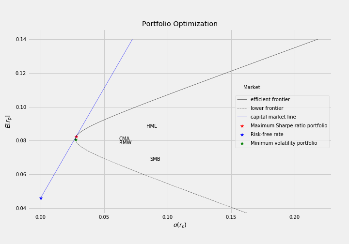
## plot the efficient frontier and capital market line 
port.display_efficient_frontier(assetsAnnotation=True, 
                                specialPortfolioAnnotation=True, 
                                addTangencyLine=True, 
                                upper_bound=0.14)

Constrained Portfolio

Let’s continue to use the FF-5 Factor data. However we are interested in a portfolio with the following constraints

\[\begin{array}{c|cc} \text{Asset} & \text{Lower Bound %} & \text{Upper Bound %}\\\ \hline \text{MKT} & 0 & 100 \\\ \text{HML} & 50 & 100\\\ \text{SMB} & 0 & 100 \\\ \text{RMW} & 0 & 100 \\\ \text{CMA} & -50 & 100 \\\ \end{array}\]

We can set up the following constraints

constraints = {'Market': [0, 1], 
               'HML': [0.5, 1], 
               'SMB': [0, 1], 
               'RMW': [0, 1], 
               'CMA': [-.5, 1]}
configuration['constraints'] = constraints
## obtain weights allocated on each asset
weights = port.get_allocations(configuration=configuration)

Black-Litterman Portfolio Allocation

Investors are interested in incorporating views, when they are solving asset allocation problems. For example,

\[\begin{array}{c|cc} \text{View} & \text{Confidence Level %} & \text{Plus and Minus %}\\\ \hline \text{Market outperforms by 1%} & 95 & 5 \\\ \text{SMB beats RMW by 1%} & 90 & 5\\\ \text{A portfolio of 20% of SMB and 80% of HML beats RMW by 1%} & 99 & 1\\\ \end{array}\]

We can use BlackLittermanPortfolio to incorporate these views

from portfolio_optimization import BlackLittermanPortfolio
## assetNames are ['Market', 'HML', 'SMB', 'RMW', 'CMA']
port = BlackLittermanPortfolio(modeledReturn, modeledCovariance, assetNames, riskFreeRate=0.046)
views = {'Market': {'type': 'absolute', 'scale': 0.01, 'confidence': 95, 'plusminus%': 5},
         'SMB|RMW' : {'type': 'relative', 'scale': 0.01, 'confidence': 90, 'plusminus%': 5, 'weights': [1., -1.]},
         'SMB|HML|RMW' : {'type': 'relative', 'scale': 0.01, 'confidence': 99, 'plusminus%': 1, 'weights': [.2, .8, -1.]},
         }
## second paramter is the R^2 used in estimating your modeled expected returns
port.update_views(views, 0.1)

## Let's use the same parameters
configuration = {'constraints': None, 
                 'riskAversion': None, 
                 'targetReturn': 0.1}
## you can obtain the BL weights                
weights = port.get_allocations(configuration=configuration)

## you can reset the portfolio to become a regular Markowitz portfolio
port.reset()

As we mentioned the \(R^2\) of the modeled returns, we will introduce some factor modeling tools in the later iteration. For beginners, let’s consider the widely used factor models, Captial Asset Pricing Model (CAPM). In general, if you use the CAPM to estimate returns, the \(R^2\) typically is below 15%. Hence, the parameter in the update_view member function would be typically set below 15% (e.g. we set at 10%).

I will add more functionality overtime. In the next iteration, I will include the following

Hansen-Jaganathan bound test
Factor Models for estimating Stochastic Discount Factors
Style Analysis

Johnew Zhang

Researcher