Project: Variational Autoencoder
- 10 minsAs images can be considered as realizations drawn from a latent variable model, we are implementing a variational autoencoder using neural networks as the variational family to approximate the Bayesian representation. Unlike the other parametric distributions, neural networks can approximate arbitrary distribution reasonably well. In this project, we are also interested in examining the effectiveness of such encoders on the SVHN dataset. By comparing different architectures, we hope to understand how the dimension of the latent space affects the learned representation and visualize the learned manifold for low-dimensional latent representations. Lastly, we will do a comparison among different variational autoencoders.
Introduction
In this article, we will discuss the methodology used to produce the variational autoencoder based on Kingma, and Welling (2014) and explore how the model performs on the MNIST and SVHN datasets. At first, it is worthwhile to summarize how the proposed methodology works and what is the intuition behind it. Before, discussing the methodology, let’s define some basic notation used in the rest of this document.
- \(X\) is the dataset we are interested in. Since we are working mostly on the image dataset, we will call \(X\) the image data.
- \(z\) is the latent state variable.
- \(p_{\phi}(z\vert X)\) is the target distribution of the latent state space.
- \(q_{\theta}(z\vert X)\) is the variational family for the latent state space.
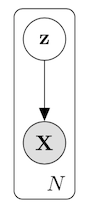
The proposed variational autoencoder is constructed on the premise that the image data is generated by some hidden features (i.e. the latent state variables). In addition, we believe the latent features for a specific set of images (e.g. a set of dog pictures) are sampled based on a prior distribution of \(z\). The following figure shows the idea.
We are interested in modeling the target distribution of the latent state space given the data \(X\), \(p_{\phi}(z\vert X)\). However, typically this distribution is not tractable so we are using the variational inference proposed in the paper. Here especially, we are performing inference using the (Kullback-Leibler) KL divergence metrics. In the rest of the report, we will discuss the methodology used in the estimation, present some results on the MNIST and SVHN datasets using different architectures, and link some potential improvements on the autoencoder.
Methodology
As discussed in the introduction, we need to do variational inference on the target distribution \(p_{\phi}(z\vert X)\). In other words, we need to pick \(q_{\theta}(z \vert X)\) from a variational family that minimizes the KL divergence metric,
\[\min D_{KL}(q_{\theta}(z\vert X)\|p_{\phi}(z\vert X))\]Based on Doersch (2016), we can have the following relationship for our KL metrics
\[\log p(X) - D_{KL}(q_{\theta}(z\vert X)\|p_{\phi}(z\vert X)) = E_q[\log p_{\phi}(X\vert z)] - D_{KL}(q_{\theta}(z\vert X)\|p(z))\]This is the core of the variational autoencoder used in the report. Since \(D_{KL}(q_{\theta}(z \vert X)\|p_{\phi}(z\vert X))\) is non-negative and, in general, needs to be minimized, the right-hand side acts as the lower bound of the log-likelihood function of the marginal image distribution. Let’s denote it as
\[\mathcal{L}(X, \phi, \theta) = E_q[\log p_{\phi}(X \vert z)] - D_{KL}(q_{\theta}(z\vert X)\|p(z))\]Intuitively, we can maximize the log-likelihood function, that is, maximize the \(\mathcal{L}(X, \phi, \theta)\). \(\mathcal{L}(X, \phi, \theta)\) consists of two parts, the reconstruction error and the KL divergence of the approximate posterior from the prior.
One can use the Monte-Carlo EM method to estimate the \(\theta\) and \(\phi\) but it can be slow. Here, we will use the stochastic gradient descent through the backpropagation in a neural network. To do this, we have to use a reparameterization trick to provide inputs \(z\) for \(p_{\phi}(X\vert z)\). Now consider two networks, the autoencoding network (encoder) and the reconstruction network (decoder). The encoder takes a set of images and outputs its hidden features; the decoder consumes some hidden features sampled from the prior distribution of the latent state variables and generates parameters in the distribution \(p_{\phi}(X\vert z)\). Kingma, Welling (2014) says the sampled input to the decoder, \(\mathbf{z}\) can be expressed as a deterministic variable \(g_{\theta}(x, \varepsilon)\), where \(\varepsilon\) is called an auxiliary variable. For example, in the univariate Gaussian case, \(\mathbf{z} = \mu + \sigma \varepsilon\), where \(\varepsilon \sim N(0, 1)\).
Gaussian Encoder
Typically, people use Gaussian as the variational inference family for Encoder distribution. In addition, we can also assume the prior distribution of the latent state model is Gaussian. Doersch (2016) derived the KL divergence of two Gaussian as following
\[\frac{1}{2}\left(tr(\Sigma\left(X, \theta)^{-1}\Sigma\right)+(\mu(X, \theta) - \mu)'\Sigma(X, \theta)(\mu(X, \theta) - \mu) - k + \log\left(\frac{\vert\Sigma(X, \theta)\vert}{\vert\Sigma\vert}\right)\right)\]where \(k\) is the dimension of the number of latent features.
If we assume the prior distribution of the latent state model is a standard multivariate Gaussian, then the KL divergence is
\[\frac{1}{2}\left(tr(\Sigma(X, \theta)) + \mu(X, \theta)'\mu(X, \theta) - k - \log\vert\Sigma(X, \theta)\vert\right)\]For the reparameterization part, we can sample from \(N(\mu(X, \theta), \Sigma(X, \theta))\) by first sampling \(\varepsilon \sim N(0, I)\) and then compute \(\mathbf{z} = \mu(X, \theta) + \Sigma(X, \theta)^{1/2}\varepsilon\). In particular, since the prior distribution of \(z\) is standard spherical Gaussian, the posterior is close to having a diagonal covariance matrix. Hence we can simplify the computation to be
\[\mathbf{z} = \mu(X, \theta) + \sqrt{tr(\Sigma(X, \theta))}\varepsilon\]Lastly, the distribution of the decoder can be chosen as either Bernoulli or Gaussian. For Gaussian, we use a diagonal matrix for its covariance matrix.
Empirical Analysis
In this section, we will discuss the details of our experiment on the MNIST and SVHN datasets respectively. As the variational autoencoder performance on MNIST dataset is generally well-behaved, we will investigate it first. Then we will discuss the effectiveness of the variational autoencoder on SVHN dataset.
MNIST Data
In the first experiment on the MNIST dataset, we used a simple fully connected neural network for the Gaussian encoder and Bernoulli decoder for various dimensionalities of the latent space. In Figure 1, we have an average result from the generative decoder based on the sample data shown in 1a. As the dimension increases in the latent space, we see a significant improvement in the decoder. In the later SVHN model, we will observe a similar behavior. In the 2 dimensional space, it appears only 0, 1, 3, 8, and 9 are recognized. In 1c, 6, and 7 get recognized. In 1d and 1e, all digits can be represented by the decoder.
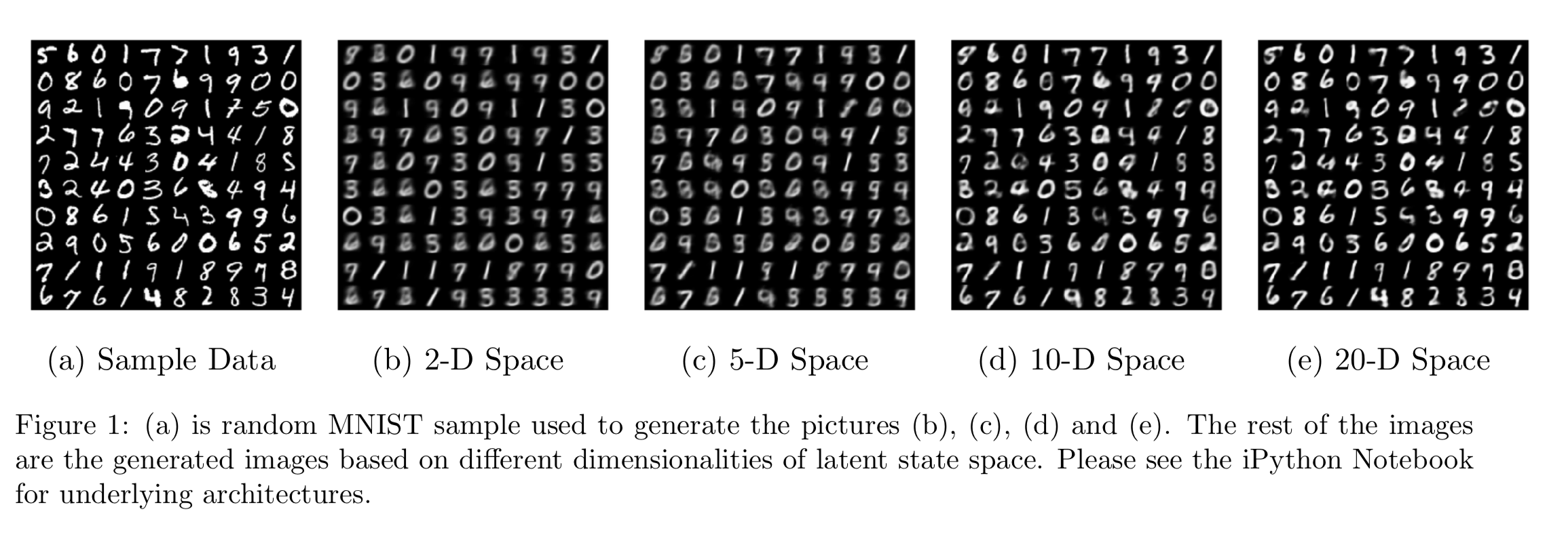
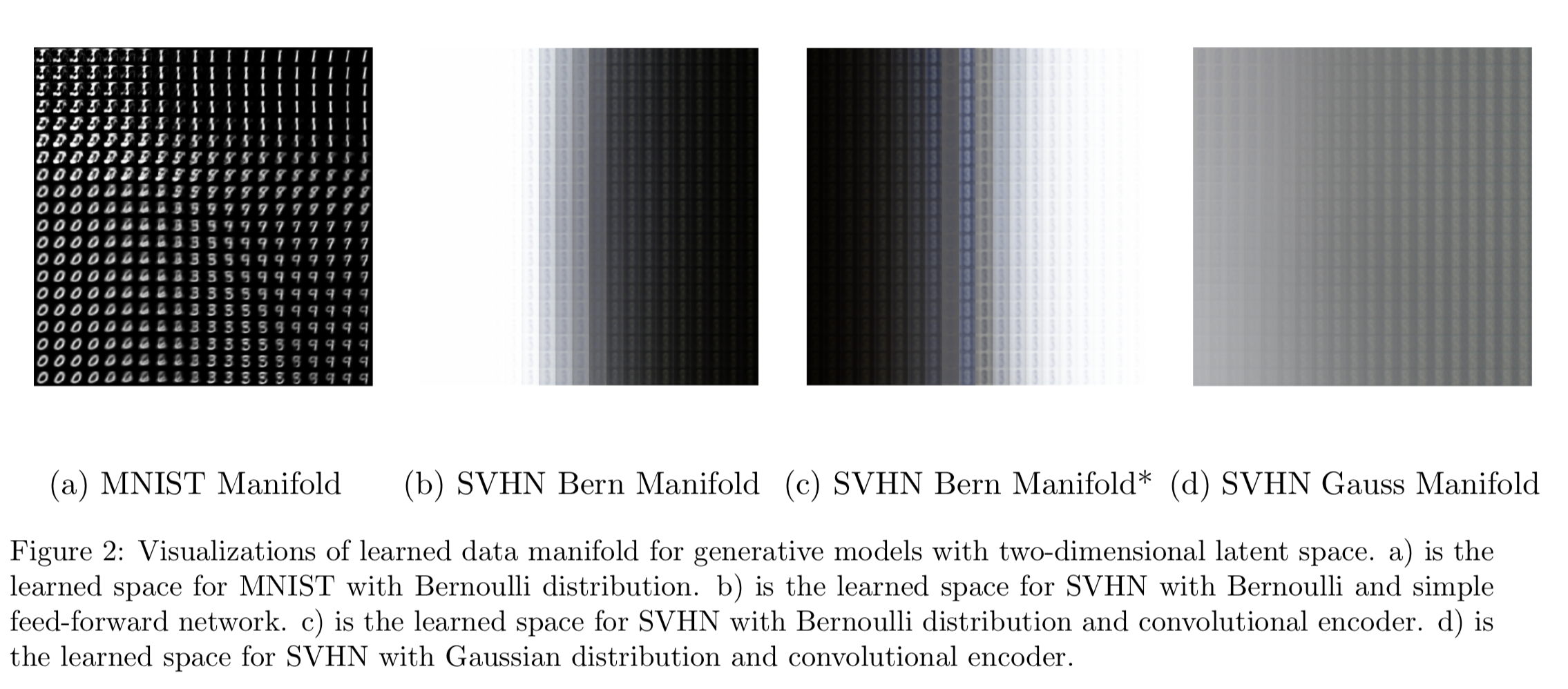
Figure 2, 2a shows the space learned by our autoencoder. It is consistent with what we see in the 2D case in Figure 1b. We know that the MNIST images are only \(28\times 28\) so it may not seem too bad to use low dimensional latent space to represent it and using a Bernoulli decoder makes sense here because the images are only black and white. Now, when we move from MNIST to SVHN, the input size is getting increased to \(32 \times 32\times 3\) (RGB images). With the complexity of images, we may not get as good representation under low-dimensional settings. In the SVHN data section, we will discuss the architectures we have looked at and how they do.
SVHN Data
It is natural to start from the model used in the MNIST case and then progress towards more complicated architectures. Hence, we will start our experiment from fully connected networks to a convolutional network.
Experiments with Bernoulli Decoder and Fully Connected Neural Network
Although the SVHN images are RGB images, pixel information is saved as between 0 and 1. Conveniently, the matplotlib library can render them into colored images. Therefore, we can still model this as a probability in the Bernoulli distribution but the representation is the relative color. Since the input size of the SVHN data is a lot larger than the MNIST, we add additional layers within the encoder and decoder in an effort to gain more complexity. First, we start with the two-dimensional manifold learned from the SVHN images (Figure 2b). The autoencoder seems to be able to pick number 8 but all the images learned are homogeneous other than the shades. In short, the features of shades and number 8 are captured by the encoder. This is a decent representation.
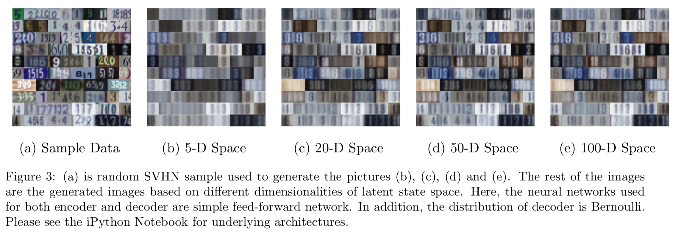
Next, we increase the dimensions of the latent space to 5, 20, 50, and 100 (the same for the rest of the discussions for SVHN). In Figure 3, 3b may validate the patterns we have seen in the low dimensional case are 8s. As the dimension rises, more colors and numbers are classified but they are still far from the sample data. In particular, the color green has not been perceived by the learner. Maybe we should try something different.
Convolutional neural networks are good at doing image processing and computer vision projects tend to use it to do image classifications. Hence, it can be a worthwhile thing to try. In all our examples below, we are only using one convolutional layer on the encoder side but not the decoder. In general, we may have decoders as mirror images of the encoder so many use deconvolutional layers to output the generated images. In addition, the training time for convolutional neural networks is typically quite long without GPU and more computing power. For simplicity, we are one convolutional layer with 16 activation maps to process the images.
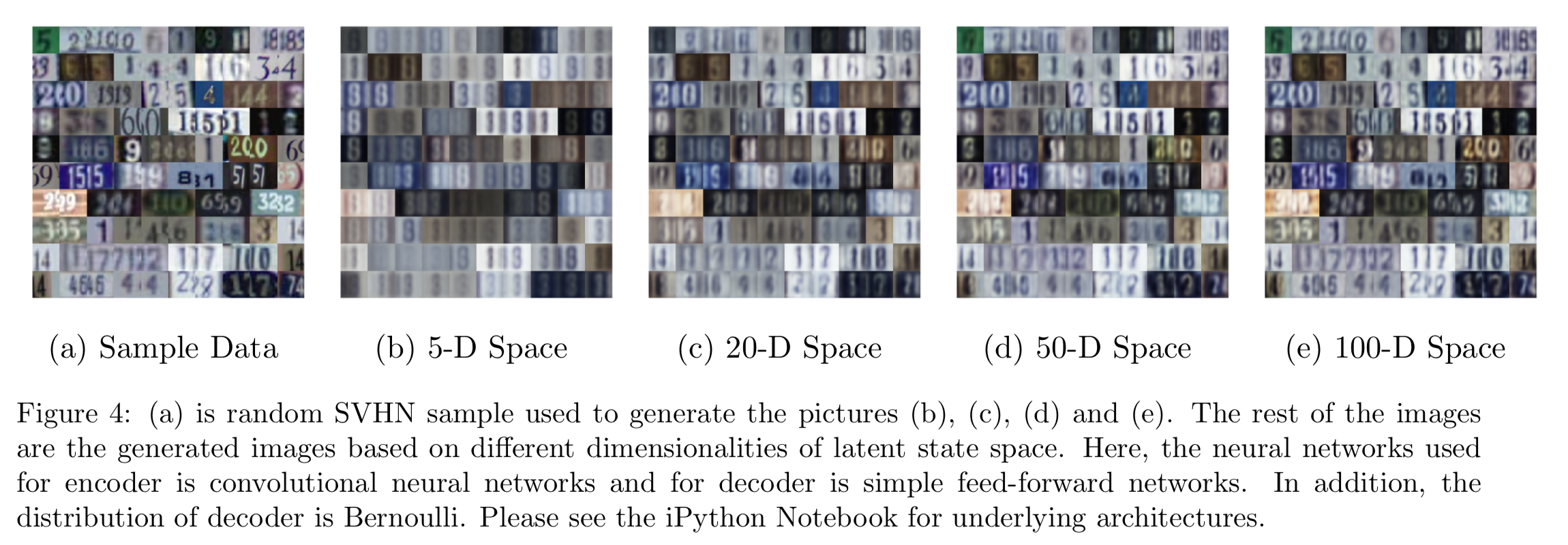
Experiments with Bernoulli Decoder and Convolutional Neural Network
Let’s continue with the Bernoulli decoder. In Figure 2c, the learned manifold looks similar to 2b. In addition, the color blue is also included. This can be considered as the feature of the color spectrum. While increasing the dimensions, we do observe the vast improvement in generated images in Figure 4. At 100D latent space, the generated images are almost the same as the sample data.
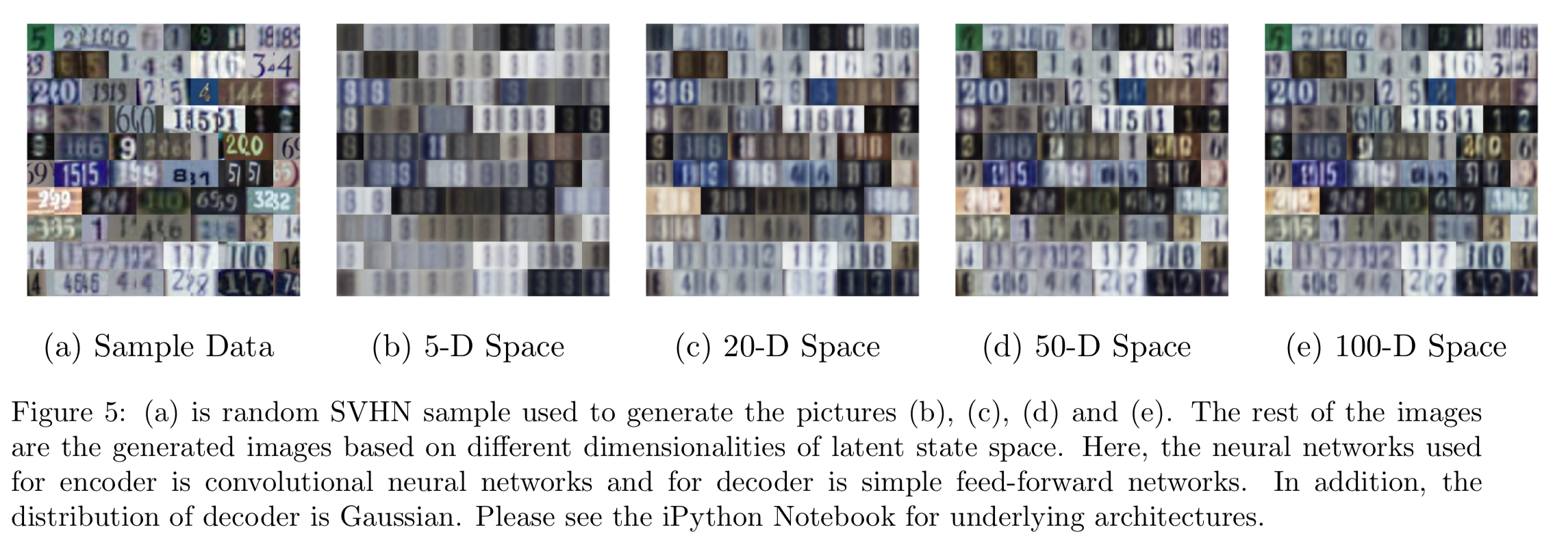
Experiments with Gaussian Decoder and Convolutional Neural Network
Lastly, since RGB is not a probability, Gaussian decoders may be more appropriate than Bernoulli decoders. From Figure 5, under the same neural network architecture, the performance is similar to the Bernoulli version so there might not be an advantage of using Gaussian. However, one issue for Gaussian is that it can produce negative means and we have to apply sigmoid functions on the means so they are forced to be between 0 and 1.
Interestingly, in Figure 2d, the learned manifold with 2 latent features under the Gaussian assumption produces more separation between light and dark colors, and the digit 8 is more apparent. It is arguable that the autoencoder with a Gaussian decoder may learn faster than the ones with Bernoulli.
Conclusion
The variational autoencoder based on Kingma, Welling (2014) can learn the SVHN dataset well enough using Convolutional neural networks. As more latent features are considered in the images, the better the performance of the autoencoders is. Lastly, a Gaussian decoder may be better than a Bernoulli decoder working with colored images.
My code is available here.
References
- [stat.ML] Diederik P. Kingma and Max Welling, Auto-Encoding Variational Bayes, 2014.
- [stat.ML] Carl Doersch, Tutorial on Variational Autoencoders, 2016.

Johnew Zhang
Researcher