Research: Essay on Asset Returns with Intertemporal CAPM
- 17 minsThis paper replicates the return decomposition methodologies proposed by Campbell and Vuolteenaho (2004) and Campbell, Giglio, Polk, and Turley (2018), which explained the size and value “anomalies” in stock returns. We show that due to the co-movement of the cash flow and discount risk in the modern period, there is little evidence that the value stocks have significantly higher betas than the growth stocks; however, the news about expected future market volatility can disentangle the size-and-value puzzle effectively. Empirically, small stocks and value stocks require less hedging premium than large and growth stocks. Lastly, their methodology shows some ability to price the abnormal returns of popular equity strategies and currency carry trade premiums.
Introduction
It is well-known that the CAPM fails to explain the stock average return in the modern period (after 1963) using the value-weighted S&P 500 return as a proxy for the market portfolio. According to Sharpe (1964) and Lintner (1965), a single total wealth portfolio can summarize a stock’s return characteristics with its beta. However, Fama and French (1995) documented the size and value anomalies and indicated that portfolios tilting towards small and value stocks tend to generate excess returns. By solving Merton (1973)’s intertemporal capital asset pricing model (ICAPM) with the Epstein and Zin (1989) utility framework of representative agents, Campbell and Vuolteenaho (2004) provided an elegant explanation by splitting the beta risk into “bad” and “good” varieties, the beta associated with the news about cash flow and the beta associated with the news about discount rate. They showed some evidence that value stocks and small stocks have considerably higher cash-flow betas than growth stocks and large stocks. In other words, for a conservative long-term investor under the ICAPM framework, small and value stocks are intertemporal hedges and perform well when investment opportunities deteriorate; however, in equilibrium, these assets should have delivered a lower average return, so the rational long-term investor should not tilt their portfolio towards small and value stocks. Furthermore, in a subsequent paper, Campbell et al. (2018) claimed that either the increasing volatility of stock returns or decreasing expected stock returns can send negative shocks to investment opportunities in the stock market. In addition to the low-frequency movements in the equity volatility, they proposed a three-beta ICAPM with the cash-flow, discount rate, and risk news to explain the cross-sectional asset return puzzle, and provided consistent results as their “Bad Beta, Good Beta” paper.
In this paper, we are interested in examining whether the two-beta ICAPM in Campbell and Vuolteenaho (2004) and three-beta ICAPM in Campbell et al. (2018) can still explain the size and value puzzle in the latest modern data (1963:07-2018:12). Under both vector- autoregressive (VAR) economies, we estimate the parameters using the full sample data (1929:06-2018:12). In the first two sections, we describe both ICAPM models and data used to estimate the parameters of VAR economies. In the third section, we walk through our estimated results of the 25 ME- and BE/ME-sorted portfolios from Ken French’s website in the modern data, and compare them against results in both Campbell’s work. In the fourth section, we conduct out-of-sample testing on some popular equity and currency trading strategies using the estimated two-beta and three-beta models. In the final section, we conclude our findings.
Model
Following Campbell and Shiller (1988), Campbell and Vuolteenaho (2004) used a log-linear approximate decomposition of returns from Campbell (1993)
\[r_{t+1} - E_tr_{t+1} = (E_{t+1} - E_t)\sum_{j=0}^{\infty}\rho^j \Delta d_{t+1+j} - (E_{t+1} - E_t)\sum_{j=0}^{\infty}\rho^j \Delta r_{t+1+j} = N_{CF, t+1} - N_{DR, t+1}\]where \(r_{t+1}\) is a log stock return, \(d_{t+1}\) is the log dividend paid by the stock, \(\Delta\) denotes a one- period change, \(E_t\) denotes a rational expectation at time \(t\), and \(\rho\) is a discount coefficient. We use \(\rho = 0.95^{1/12}\) through the entire paper. \(N_{CF}\) denotes news about future cash flow and \(N_{DR}\) denotes news about future discount rates. They assume the data are generated by a first-order VAR model
\[z_{t+1} = a + \Gamma z_t + u_{t+1}\]where \(r_{t+1}\) is the first element of \(z_{t+1}\). Provided the above process, we can obtain the news about cash flow and discount rates as follows:
\[N_{CF, t+1} = (e_1'+e_1'\lambda)\mu_{t+1}\] \[N_{DR, t+1} = e_1'\lambda \mu_{t+1}\]where \(\lambda = \rho \Gamma(I-\rho\Gamma)^{-1}\) and \(e_1\) is a vector where the first element is 1 and everywhere else is 0. As a result, the two-beta ICAPM is
\[E_t[R_{i, t+1} - R_{j, t+1}] = \gamma Cov_t[r_{i, t+1} - r_{j, t+1}, N_{CF, t +1}] + Cov_t[r_{i, t+1} - r_{j, t+1}, -N_{DR, t +1}]\]Campbell et al. (2018) argued when having the log stochastic discount factor of the intertemporal CAPM that allows for stochastic volatility, the pricing kernel has three factors
\[m_{t+1} - E_tm_{t+1} = -\gamma N_{CF, t+1} - [-N_{DR, t+1}] + \frac{1}{2} N_{RISK, t+1}\]where \(N_{RISK, t+1}\) is news about volatility. Following this fact, they assumed the economy is described by a first-order VAR
\[z_{t+1} = a + \Gamma z_t + \sigma_tu_{t+1}\]where the first two elements of \(z_{t+1}\) are \(r_{t +1}\) and \(\sigma_{t+1}^2\). They also assume that \(u_{t+1}\) has a constant variance-covariance matrix \(\Sigma\), with element \(\Sigma_{11}=1\), and \(\sigma_t^2\) is equal to the conditional variance of market returns. Given this structure, news about discount rates can be written as
\[N_{DR, t+1} = e_1'\lambda\sigma_t\mu_{t+1}\]while implied cash-flow news is
\[N_{CF, t+1} = (e_1'+e_1'\lambda)\sigma_t\mu_{t+1}\]Their specification also provides the news about risk is proportional to news about market return variance, \(N_V\):
\[N_{RISK, t+1} = \omega\rho e_2'(I-\rho\Gamma)^{-1}\sigma_tu_{t+1} = \omega N_{V, t+1}\]Hence, they derived the three-beta ICAPM model:
\[E_t[R_{i, t+1} - R_{j, t+1}] = \gamma Cov_t[r_{i, t+1} - r_{j, t+1}, N_{CF, t +1}] + Cov_t[r_{i, t+1} - r_{j, t+1}, -N_{DR, t +1}]-\frac{1}{2}\omega Cov_t[r_{i, t+1} - r_{j, t+1}, N_{V, t +1}]\]Beta Measurement
To be consistent with the previous paper in Campbell (1993), we define the betas as follows:
\[\beta_{i, CF} \equiv \frac{Cov(r_{i, t}, N_{CF, t})}{Var(r_{M, t} - E_{t-1} r_{M, t})}\] \[\beta_{i, DR} \equiv \frac{Cov(r_{i, t}, -N_{DR, t})}{Var(r_{M, t} - E_{t-1} r_{M, t})}\] \[\beta_{i, V} \equiv \frac{Cov(r_{i, t}, N_{V, t})}{Var(r_{M, t} - E_{t-1} r_{M, t})}\]and estimate the betas with a lag
\[\widehat{\beta}_{i, CF} = \frac{Cov(r_{i, t}, N_{CF, t})}{Var(N_{CF, t} - N_{DR, t}+ I_{V}N_{V, t})}+\frac{Cov(r_{i, t}, N_{CF, t-1})}{Var(N_{CF, t} - N_{DR, t}+ I_{V}N_{V, t})}\] \[\widehat{\beta}_{i, DR} = \frac{Cov(r_{i, t}, -N_{DR, t})}{Var(N_{CF, t} - N_{DR, t}+ I_{V}N_{V, t})} +\frac{Cov(r_{i, t}, -N_{DR, t-1})}{Var(N_{CF, t} - N_{DR, t}+ I_{V}N_{V, t})}\] \[\widehat{\beta}_{i, V} = \frac{Cov(r_{i, t}, N_{V, t})}{Var(N_{CF, t} - N_{DR, t}+ I_{V}N_{V, t})} + \frac{Cov(r_{i, t}, N_{V, t-1})}{Var(N_{CF, t} - N_{DR, t}+ I_{V}N_{V, t})}\]where \(I_V = 1\) if we are using three beta model; else, \(I_V = 0\). According to Campbell, they include one lag of the market’s news terms in the numerator because during the early sample period, not all stocks in their test-asset portfolios were traded frequently and synchronously.
Data Description
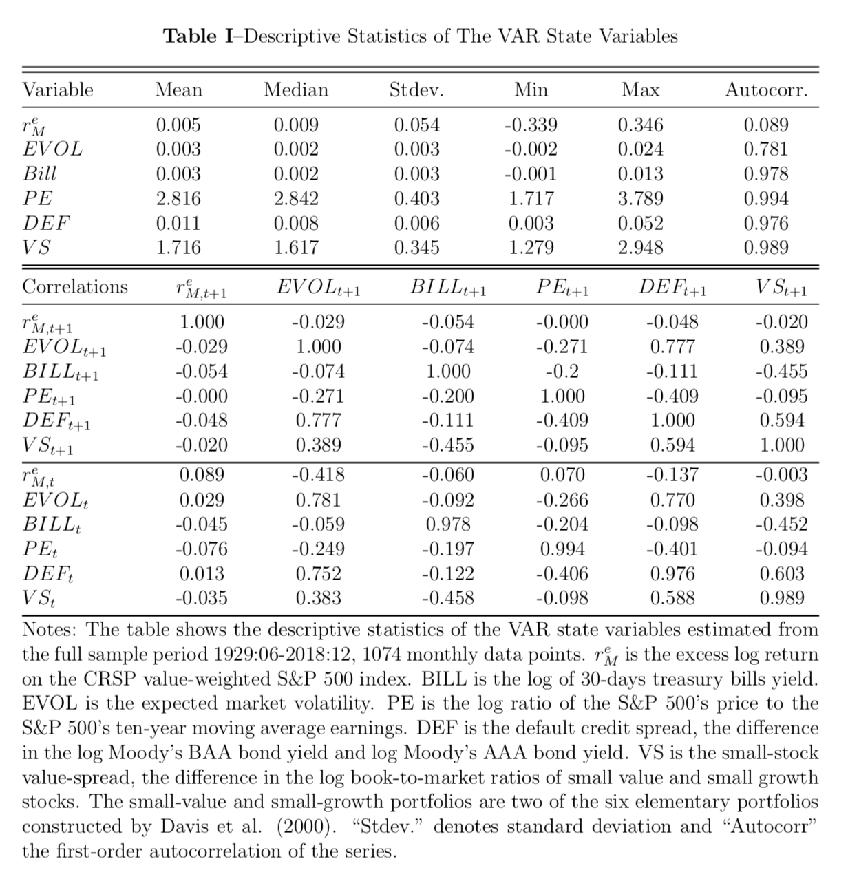
In our VAR economy, we have six state variables: the excess market return (measured as the log excess return on the Center for Research in Security Prices (CRSP) S&P value- weighted index over 30-day treasury bills); the expected market volatility, estimated using a lagged regression model; the log yield of the 30-day treasury bill; the market’s smoothed price-earning ratio (measured as the log ratio of the S&P 500 price index to a ten-year moving average of S&P 500 earnings from Schiller’s website); the default credit spread (the log yield spread between the Moody’s BAA bonds and AAA bonds, obtained from the Federal Reserve Bank of St. Louis, Missouri); and the small-stock value spread (measured as the difference between the log book-to-market ratios of small value and small growth stocks).
Campbell et al. (2018) argued that the stochastic volatility on the market makes a significant contribution to explain the cross-sectional risk premia of asset prices. They introduced the expected market volatility term (EVOL), which is meant to capture the variance of the market returns, \(\sigma_t^2\), conditional on information available at time \(t\). To construct the \(EVOL_t\), we first create a series of the within-monthly realized variance of daily returns for each time \(t\), \(RVOL_t\). We run a regression of \(RVOL_{t+1}\) on lagged realized variance as well as the rest of state variables at time \(t\) The predicted value from this regression is defined as the expected market variance (\(EVOL_t\equiv \widehat{RVOL}_{t+1}\)). Campbell et al. (2018) also included the default spread (DEF) due to the fact that it is known to track time-series variation in expected real returns on the market portfolio and shocks to the DEF should reflect news about aggregate default probabilities. Lastly, the value spread is shown by Brennan, Wang, and Xia (2004) to be predictable about future market returns. Table I reports the descriptive sample statistics on the monthly VAR state variable data between 1929:06 and 2018:12.
Results
VAR Estimates
Table II and IV report parameter estimates for the two-beta and three-beta VAR model respectively over our full sample period June 1929 to June 2018. In the two-beta model, we exclude the expected market volatility to keep it consistent with Campbell and Vuolteenaho (2004) formulation; in the three-beta model, all state variables are used. Ordinary least squares (OLS) standard errors are reported in the parentheses below the coefficients. Finally, we report the \(R^2\) for each regression. In both tables, they show the lagged market excess return together with other state variables provide some ability to predict the future market return; the term yield spread and the small value spread have a consistent coefficient as the results in Campbell and Vuolteenaho (2004). Campbell et al. (2018) shows the expected volatility and the default credit spread positively predict the excess return. Our default credit spread has a negative sign in the three-beta VAR economy but insignificant. We can argue that the market volatility tends to widen the credit spread so the EVOL have explained the majority of the default spread, so the negative contribution from DEF provides some offsetting effect. The smoothed price-earning ratio shows a negative predictive power. Overall, about 2 percent \(R^2\) of both forecasting models is reasonable for monthly return model.
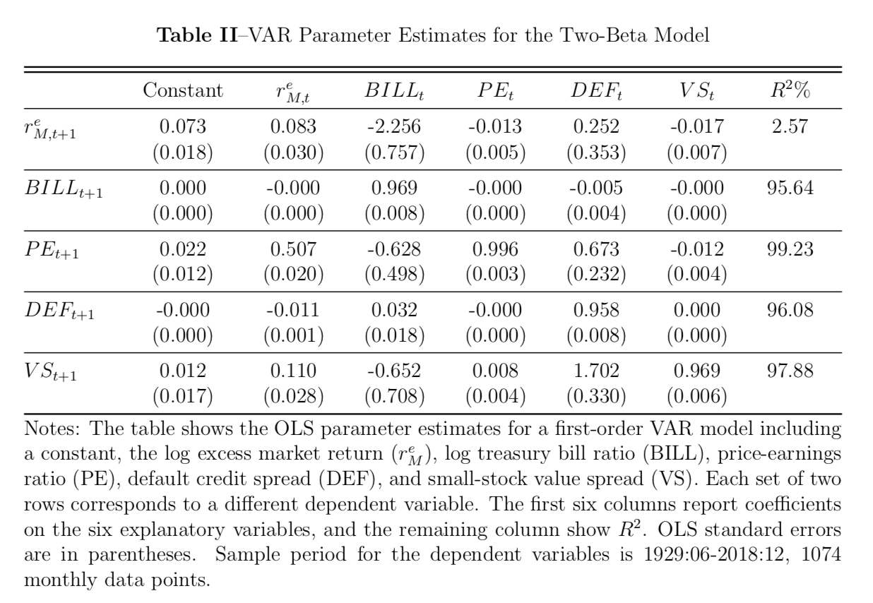
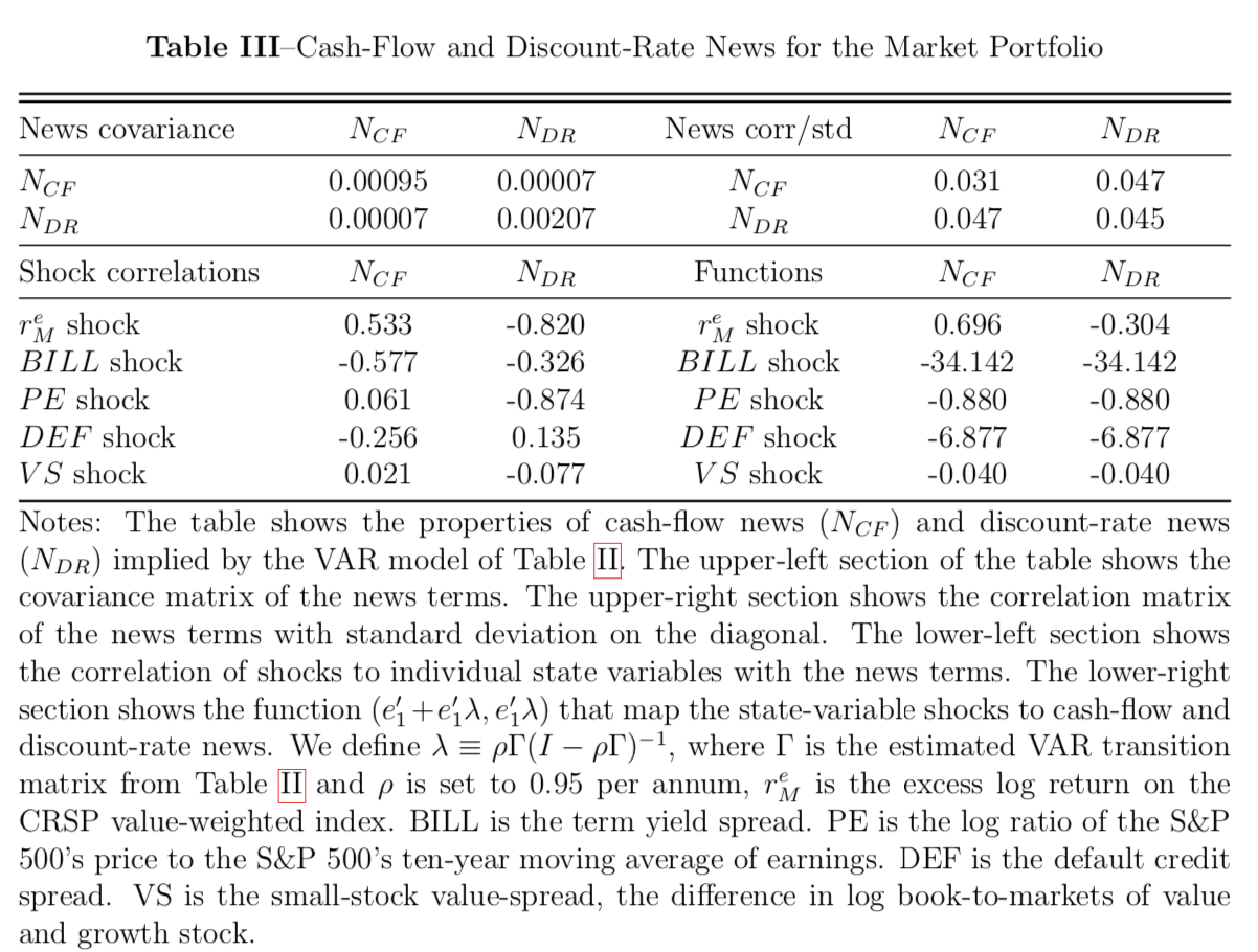
Table III and Table V summarize the behaviors of implied news from cash flow and discount rate from the two-beta model and implied news from cash flow, discount rate, and volatility from the three-beta model respectively. Our news from cash flow has a lower variance than one of the news from discount rate, which agrees with the finding of Campbell (1991) that discount-rate news is the dominant component of the market return.
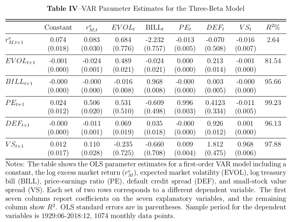
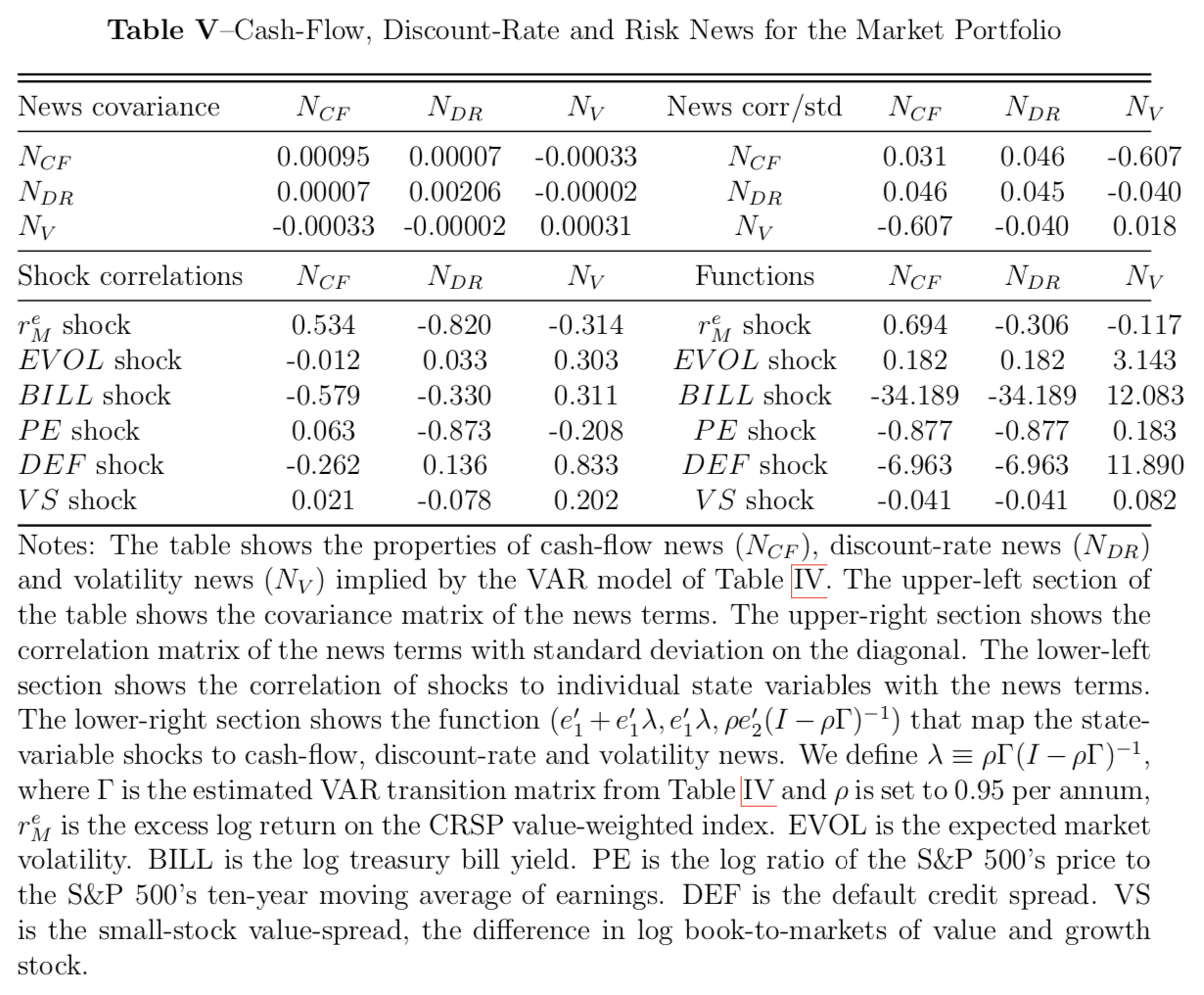
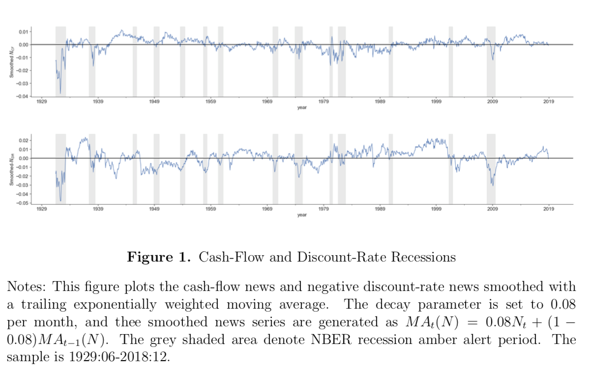
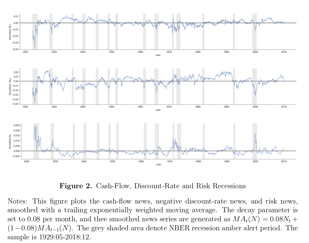
Figure 1 and Figure 2 illustrate the VAR model’s view of stock market history related to NBER recessions. The shaded area indicates the amber recession alert period. Our results are similar to Campbell’s in the common period (1963-2001); during the 2008 financial crisis, we see both news about discount rates and cash flow dropped significantly. Campbell and Vuolteenaho (2004) call this as “mixed recession” (i.e. the Great Depression). In particular, the news of volatility peaked substantially in 2008.
Betas
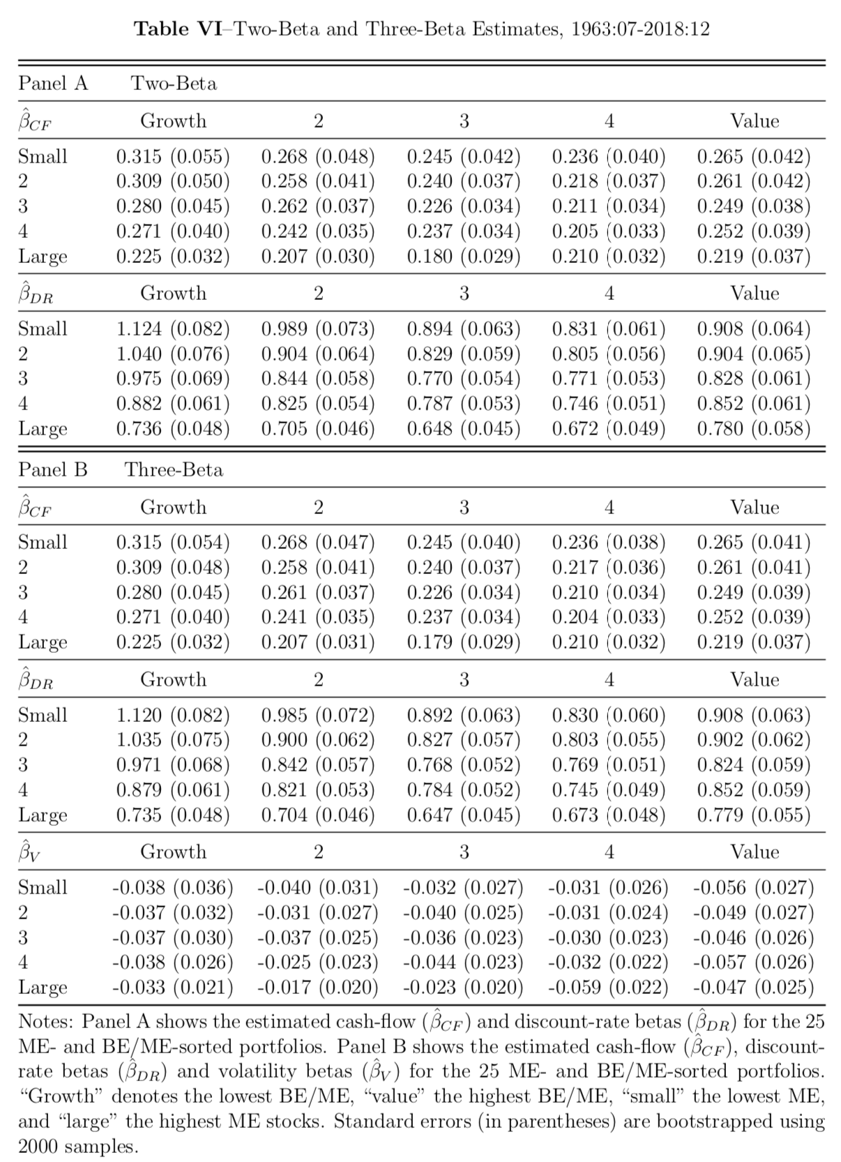
Table VI reports beta estimates for the 25 size- and book-to-market portfolios over the 1963-2018 period under both the two-beta (Panel A) and three-beta (Panel B) ICAPMs. The portfolios are organized in a square matrix with growth stocks at the left, value stocks at the right, small stocks at the top, and large stocks at the bottom. For each panel, the first matrix displays the cash-flow betas, and the second matrix displays the discount-rate betas. In Panel B, the last matrix is the estimated betas for the news about volatility. First of all, It is not a surprise to see the cash flow betas are significantly lower than the discount rate betas because cash-flow news is from the VAR economies with limited forecastability. In Panel B, since the excess return should include a volatility term (Jensen’s inequality term) as a precautionary saving motive, the negative beta estimates align with the idea that a hedging premium is paid for the news on volatility. For both ICAPMs, the small stocks still show higher betas in both discount rate and cash flow. Moreover, the value stocks show lower discount-rate betas. However, the value stocks have lower cash-flow betas than the growth stocks. This suggests that the two innovations co-move in the modern period and the two-beta model may have trouble with disentangling the size-value puzzle. Based on the three-beta ICAPM, the volatility betas from our estimates are consistent with the story from the earlier sample in Campbell et al. (2018). We may explain the lower hedging premium required for both small and value stocks gives rise to the size-and-value anomalies in the modern period.
Empirical Estimates of Risk Premia
Lastly, with the estimated betas, we can run our cross-sectional regressions
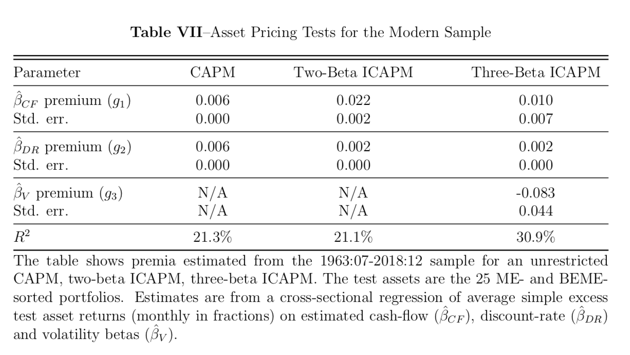
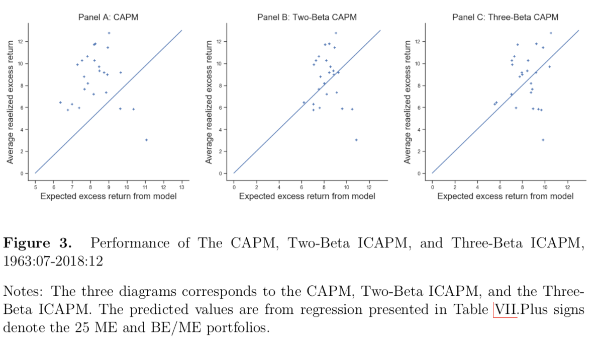
\[\bar{R}_i^e = g_1\widehat{\beta}_{i, CF} + g_2\widehat{\beta}_{i, DR} + e_i\] \[\bar{R}_i^e = g_1\widehat{\beta}_{i, CF} + g_2\widehat{\beta}_{i, DR} + g_3\widehat{\beta}_{i, V} + e_i\]respectively, where \(\bar{R}_{i}^e\equiv \bar{R}_i -\bar{R}_{rf}\) denotes the sample average simple excess return on asset \(i\). The implied risk-aversion coefficient can be recovered by \(g_1/g_2\). Table VII shows that traditional CAPM and two-beta ICAPM explain the cross-sectional variations fairly. In the earlier subsection, it suggests that the innovations from the cash-flow and discount rate co-moves in the majority of the updated period (2001-2018), especially during the financial crisis, so we can expect the two-beta ICAPM’s performance to fall off. Encouragingly, the three-beta ICAPMs explain more than 30% of the variation in the cross-section average excess returns. The two-beta ICAPM has an implied risk aversion of 12.31, while the three-beta ICAPM shows 5.25. A visual summary of these results is provided in Figure 3, where we multiply 1,200 on the estimate to show the annualized return percentage point.
Price Some Popular Equity and Currency Strategies
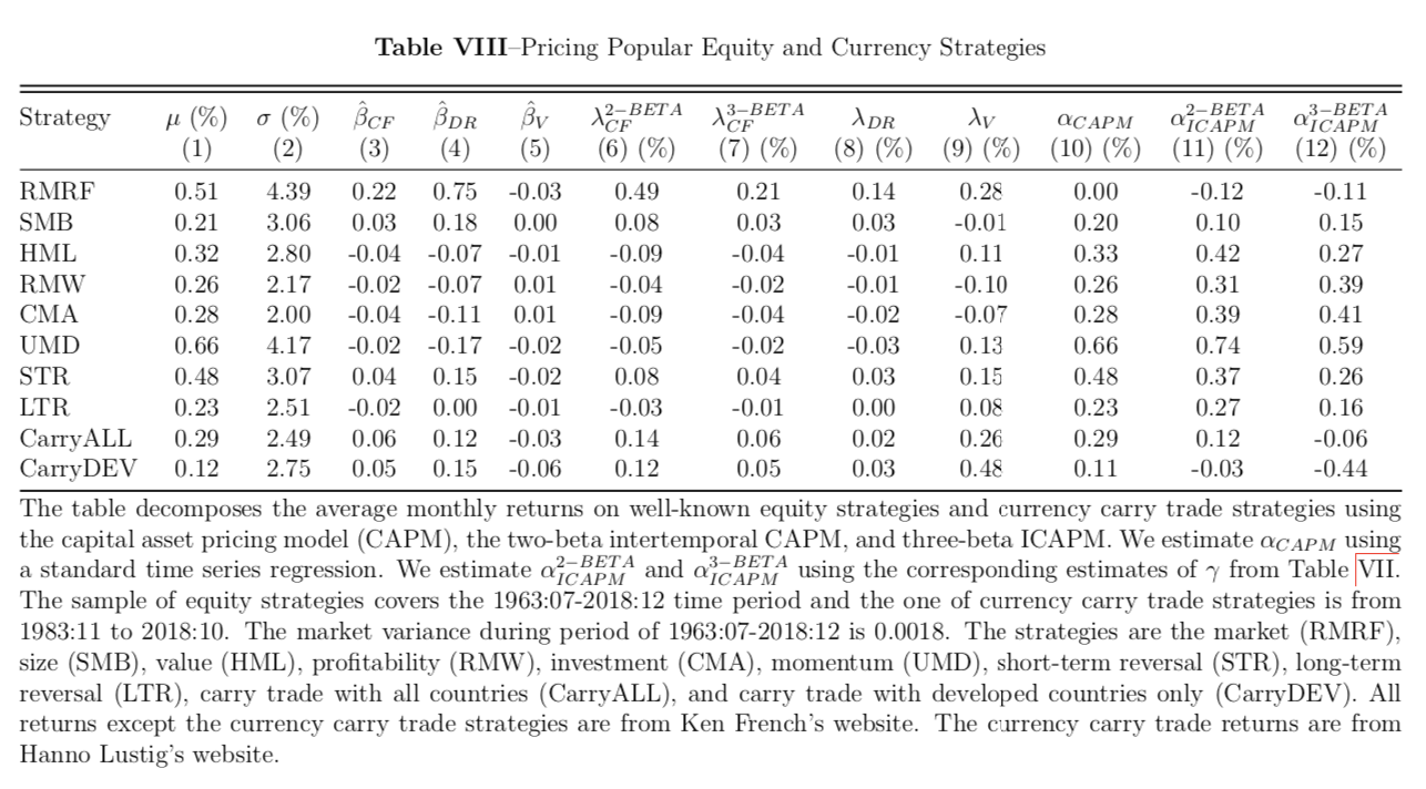
In this section, we use our ICAPM model to assess some common anomalies that have been discussed in the asset pricing literature. Table VIII analyzes several well-known equity anomalies using data taken from Kenneth French’s website. The sample period is 1963:07-2018:12. The anomaly portfolios are the market (RMRF), size (SMB), and value (HML) factors discussed in this paper, the profitability (RMW) and investment (CMA) added in Fama and French (2015), the momentum (UMD) factor of Carhart (1997), short-term reversal (STR) and long-term reversal (LTR) factors. We also include the currency carry trade long-short portfolio strategies proposed in Lustig, Roussanov, and Verdelhan (2011) with all countries and developed countries only. For each of these portfolios, Table VIII reports the mean excess return in the first column and the standard deviation of return in the second column. Column 3-5 report the portfolios’ betas with our estimates of discount-rate news, cash-flow news, and volatility news. These are used in Column 6-9 to construct the components of fitted excess returns based on discount-rate news (\(\lambda_{DR}\)), cash-flow news in the two-beta ICAPM (\(\lambda^{2−BETA}_{CF}\)), cash-flow news in the three-beta ICAPM (\(\lambda^{3−BETA}_{CF}\)), and the variance news in the three-beta ICAPM (\(\lambda_V\)). These fitted excess returns use the parameter estimates of the two-beta and three-beta models reported in Table VII. We do not reestimate any parameters so we can think of this analysis as an out-of-sample test. Columns 10-12 report the alphas of the anomalies (their sample average excess returns less their predicted excess returns) calculated using the CAPM, the two-beta ICAPM, and the three-beta ICAPM. All the portfolios, with the obvious exception of RMRF, have been chosen to have positive CAPM alphas.
Table VIII shows that the volatility risk exposure explains the majority of abnormal returns. Most of the anomaly portfolios have negative betas on the volatility news, which makes them riskier and helps to explain their positive excess returns. The exceptions are SMB, RMW, and CMA portfolios. Here, the two beta model is not necessarily better than the CAPM, but it does explain well the developed country carry trade return. Against the two-beta ICAPM, the three-beta ICAPM shows a much more promising interpretation of the value and size portfolio returns. Interestingly, the three-beta model shows a better result in explaining the carry trade return with all countries. It indicates that the carry premium arises from the volatility news in the US equity markets. Overall, the three-beta model gives a more accurate prediction than the CAPM and the two-beta ICAPM.
Conclusions
Empirically, we find that value stocks and small stocks have considerably lower insurance premiums to hedge future volatility shock, and this can explain their higher average returns. However, we cannot find clear higher cash-flow betas in both two-beta and three-beta ICAPMs. Chen and Zhao (2009) argued news about cash flow is computed residually relative to the news about the discount rate, so the cash-flow news captures all the noise in the VAR model. If a variable is omitted from it, but it belongs to rational investors’ information set, it ends up in the innovation of the cash-flow news. Therefore, the cash-flow news is really sensitive to the VAR specification. They showed that value companies do not have larger cash-flow betas with alternative VAR specifications. This is consistent with our beta estimates. Hence, the disagreement on cash-flow betas may stem from the misspecification of the VAR economies.
References
- Brennan, Michael J., Ashley W. Wang, and Yihong Xia, 2004, Estimation and test of a simple model of intertemporal capital asset pricing, The Journal of Finance 59, 1743–1776.
- Campbell, John, 1993, Intertemporal asset pricing without consumption data, American Economic Review 83, 487–512.
- Campbell, John Y., 1991, A variance decomposition for stock returns, The Economic Journal 101, 157–179.
- Campbell, John Y., Stefano Giglio, Christopher Polk, and Robert Turley, 2018, An intertemporal CAPM with stochastic volatility, Journal of Financial Economics 128, 207–233.
- Campbell, John Y., and Robert J. Shiller, 1988, The dividend-price ratio and expectations of future dividends and discount factors, The Review of Financial Studies 1, 195–228.
- Campbell, John Y., and Tuomo Vuolteenaho, 2004, Bad Beta, Good Beta, American Economic Review 94, 1249–1275.
- Carhart, Mark M., 1997, On persistence in mutual fund performance, The Journal of Finance 52, 57–82.
- Chen, Long, and Xinlei Zhao, 2009, Return decomposition, The Review of Financial Studies 22, 5213–5249.
- Epstein, Larry G., and Stanley E. Zin, 1989, Substitution, risk aversion, and the temporal behavior of consumption and asset returns: A theoretical framework, Econometrica 57, 937–969.
- Fama, Eugene F., and Kenneth R. French, 1995, Size and book-to-market factors in earnings and returns, The Journal of Finance 50, 131–155.
- Fama, Eugene F., and Kenneth R. French, 2015, Dissecting Anomalies with a Five-Factor Model, The Review of Financial Studies 29, 69–103.
- Lintner, John, 1965, The valuation of risk assets and the selection of risky investments in stock portfolios and capital budgets, The Review of Economics and Statistics 47, 13–37.
- Lustig, Hanno, Nikolai Roussanov, and Adrien Verdelhan, 2011, Common Risk Factors in Currency Markets, The Review of Financial Studies 24, 3731–3777.
- Merton, Robert, 1973, An intertemporal capital asset pricing model, Econometrica 41, 867– 87.
- Sharpe, William F., 1964, Capital asset prices: A theory of market equilibrium under the condition of risk, The Journal of Finance 19, 425–442.

Johnew Zhang
Researcher